Servo Motor Working Principle Explained: Three-Loop Control (Current/Velocity/Position Loop) and Stiffness Tuning

The servo motor principle in one sentence: the motor itself knows where it has rotated to. The encoder at the rear continuously reports position, and the driver compares the reported value with the command and corrects the current in real time — this "command → feedback → correction" closed loop is the most fundamental difference between servo control and ordinary motor drive.

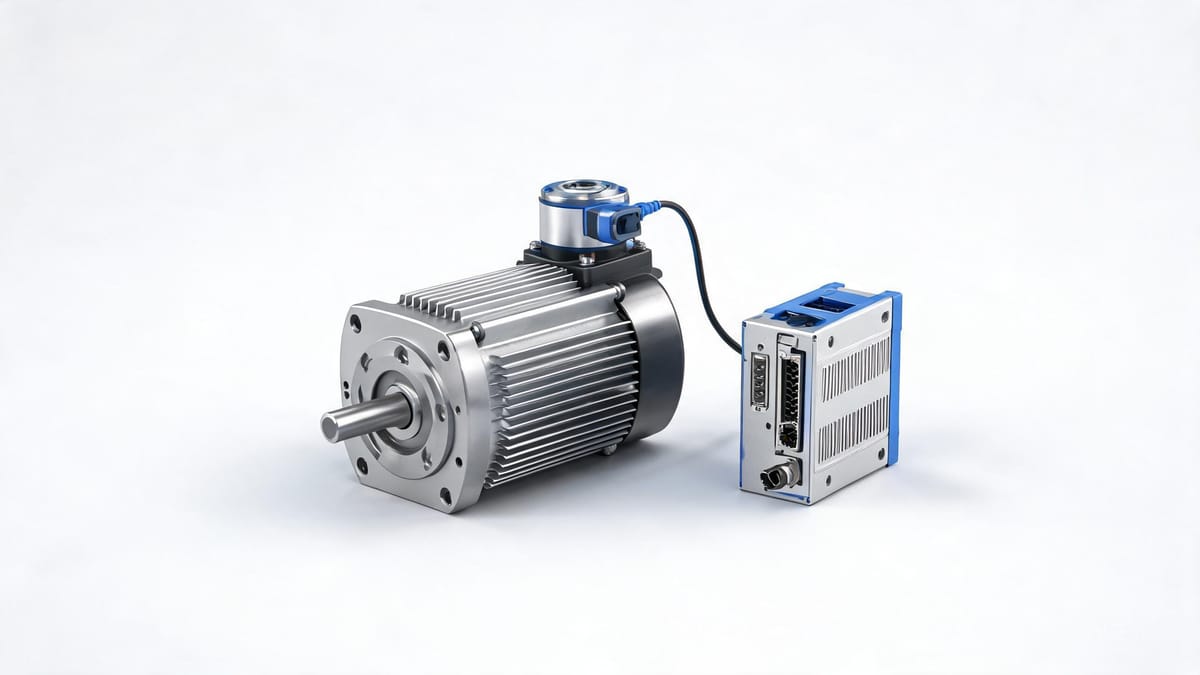
Figure: Servo motor with high-resolution encoder — the encoder reports position in real time, forming a "command → feedback → correction" closed loop

1. What Is a Servo System

Definition

A servo system is an automatic control system that makes the output controlled quantity of an object's position, orientation, state, etc., follow any change of the input target (or setpoint).

Composition

A servo system consists of three parts:

1. Controller (host PLC / motion controller / CNC) → sends commands

2. Actuator (servo driver + servo motor) → delivers force

3. Controlled object (mechanical load) + feedback device (encoder) → reports the actual state

The word "Servo" comes from the Latin servus (slave) — the output faithfully follows the command; this is the essence of servo.

Three Core Parts

Opening up a modern servo motor, the core is just three things:

2. Three-Loop Control: The Core of the Servo Driver

The control core of a servo driver is a cascade control system, with three loops nested from inner to outer:

Position loop (outermost, decides "where to go")
  Input: target position   Feedback: encoder position   Output: velocity command
        ↓
Velocity loop (middle, decides "how fast")
  Input: velocity command   Feedback: encoder velocity   Output: current/torque command
        ↓
Current loop (innermost, decides "how hard to push")
  Input: current command   Feedback: current sensor   Output: PWM voltage
        ↓
      Drives the motor to produce torque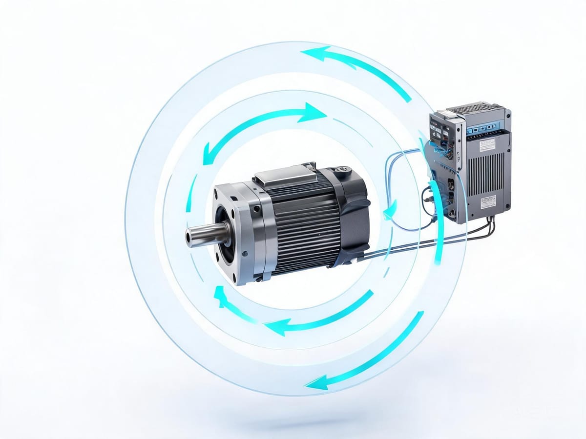

Figure: Three-loop cascade control — position, velocity and current loops nested from outer to inner

Current Loop: Innermost, Fastest

Function: controls the winding current, and current × torque constant = output torque. It is the fastest, highest-bandwidth loop of the three and determines the system's "explosive power."

Features:

• Performed entirely inside the servo driver; PID constants are set by the manufacturer and users do not need to change them;

• Feedback comes from the per-phase Hall elements or sampling resistors inside the driver;

• Its function is PD/PID regulation of the difference between input and feedback values;

• It suppresses starting/braking current surges, accelerates the current response, and provides overcurrent protection.

Modern implementation: FOC vector control

Modern servos generally use Field-Oriented Control (FOC), which through the Clark transform (three-phase stationary → two-phase stationary) and the Park transform (two-phase stationary → two-phase rotating d-q coordinates) converts complex AC motor control into simple DC-motor-like control: Id controls excitation, Iq controls torque. An inverse Park transform then generates the SVPWM modulation signal.

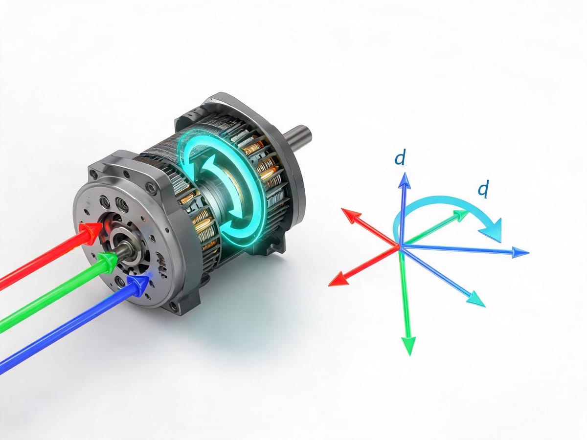
Figure: FOC field-oriented control — converts AC motor control into decoupled DC-motor-like control through coordinate transformation

Typical cycle: 50–100 μs (10–20 kHz)

Fault clue: current-loop oscillation usually appears as high-frequency whistling (>1 kHz), possibly caused by excessive current-sampling noise, improper PWM dead-time settings, or reflected voltage from an overly long motor cable.

Velocity Loop: The Commander of Dynamic Response

Function: receives the velocity command from the position loop and, by adjusting the current command, makes the motor's actual speed track the target quickly and without overshoot.

Features:

• Uses PI regulation (proportional + integral);

• Feedback is the actual speed computed from the encoder signal by the "velocity calculator";

• By adjusting gain and integral time constant, it suppresses oscillation, reduces overshoot, and improves system responsiveness;

• Its output is the setpoint of the current loop.

Typical cycle: 200–500 μs (2–5 kHz)

Relationship between bandwidth and stiffness:

Kv = J × ωbw (velocity loop gain = load inertia × bandwidth)

Mechanical resonance trap: when the velocity loop bandwidth approaches the mechanical system's natural frequency, resonance occurs. Typical symptoms are abnormal vibration in a specific speed range, speed-dependent whistling, and persistent jitter after positioning completes.

Solutions:

1. Notch filter: deep attenuation at the resonance frequency;

2. Low-pass filter: reduce velocity loop bandwidth, trading responsiveness for stability;

3. Inertia identification and adaptive control: adjust gain in real time to match load changes.

Position Loop: The Final Gatekeeper of Accuracy

Function: detects whether the motor has moved to the commanded position after the controller outputs the position command.

Features:

• Uses P regulation (proportional);

• Feedback is the residual pulses computed by the "deviation counter" from the encoder feedback pulses;

• Its output is the setpoint of the velocity loop;

• The higher the gain, the shorter the positioning time and the faster the response, while also guaranteeing steady-state accuracy.

Typical cycle: 500 μs–1 ms (1–2 kHz)

Physical meaning of position loop gain: the position loop gain Kp (unit 1/s) directly determines system stiffness:

Position following error = velocity command / Kp

Example: with Kp = 50 Hz and running speed 1000 rpm (about 104.7 rad/s), the theoretical following error = 104.7 / 50 = 2.09 rad.

Feedforward control: breaking through the feedback limit

Feedback control alone cannot eliminate following error; introducing feedforward enables "prediction":

Total output = position loop output (feedback control) + velocity feedforward + acceleration feedforward

• Velocity feedforward: directly adds the velocity command, eliminating steady-state following error;

• Acceleration feedforward: compensates for system inertia, reducing error during the acceleration segment.

Tuning tip: gradually increase the feedforward coefficient to 95%, leaving the remaining 5% to be corrected by feedback control, balancing responsiveness and stability.

3. Core Laws of Three-Loop Coordination

Bandwidth Hierarchy Principle

Current loop bandwidth > 5 × velocity loop bandwidth > 5 × position loop bandwidth

Typical configuration: current loop 2 kHz → velocity loop 400 Hz → position loop 80 Hz.

Consequence of violation: if the velocity loop bandwidth approaches the current loop, the phase lag of the current loop causes the velocity loop to oscillate. This is the root cause of "the more you tune the gain, the worse it gets."

Standard Tuning Order

Practical shortcut: the auto-tuning function of modern drivers measures load inertia and automatically configures the three-loop parameters. For general applications, run auto-tuning first, then fine-tune manually if needed.

4. Stiffness, Inertia and Resonance: Three Concepts You Must Understand

4.1 Motor Stiffness

Motor stiffness is the motor shaft's ability to resist external torque disturbance, i.e., the self-locking capability of the motor rotor.

From the controller's perspective, stiffness is actually a parameter group combining the velocity loop, position loop, and time integral constants; its magnitude determines the mechanical response speed:

• Higher stiffness → larger corresponding velocity loop gain → higher response speed;

• But too high easily causes motor resonance.

Typical phenomenon: after the positioning command ends, even if the motor itself is nearly stationary, the mechanical transmission end still shows persistent swinging.

Rigid connection vs flexible connection:

• Connecting motor and load with a coupling → rigid connection;

• Connecting motor and load with a timing belt or belt → flexible connection.

A flexible connection has low system stiffness, so the velocity loop gain must be tuned lower accordingly, otherwise oscillation is very likely.

4.2 Moment of Inertia and Torque

Inertia is a measure of the magnitude of inertia. For a rigid body rotating about an axis:

I = m · r²

The relationship between moment of inertia and torque:

M = I · β (torque = moment of inertia × angular acceleration)

The purpose of calculating load inertia is to calculate the acceleration/deceleration torque. Every rotating object has inertia; the magnitude of inertia directly reflects the torque required and the time needed for acceleration/deceleration during rotation.

4.3 Load Inertia Ratio

Load inertia ratio = load inertia / motor inertia

• Motor inertia refers to the rotor's own inertia, divided into large, medium, and small grades. From a response perspective, the rotor inertia should be small; from a load perspective, the larger the rotor inertia the better (stronger disturbance resistance);

• Load inertia consists of the inertia of linear and rotary moving parts such as the worktable, fixtures and workpieces, screw, and coupling, reflected to the motor shaft;

• The applicable load inertia is usually less than 5 times the servo motor inertia; it is generally considered large when the load inertia exceeds 10 times the motor rotor inertia;

• Above 10 times, the system responds sluggishly and is difficult to tune; you should enlarge the motor or add a planetary gearbox (inertia decays by the reduction ratio i²).

5. Three Control Modes of a Servo Motor

Additional modes:

• Full closed-loop mode: uses a linear scale feedback instead of the encoder, compensating for screw backlash;

• Interpolation mode: electronic gearing / electronic cam, for multi-axis synchronization (e.g., flying shear, rotary cut).

Key setting in position mode — the electronic gear ratio: in position mode, you must first set the electronic gear ratio based on the mechanical conditions, considering both accuracy and speed requirements, then calculate the pulse frequency and pulse count.

6. Fault Diagnosis: Infer the Loop from the Symptom

Oscilloscope diagnostic method:

• Current command vs actual current → verify current loop response speed;

• Velocity command vs actual velocity → evaluate velocity loop bandwidth;

• Position command vs actual position → check following error and overshoot;

• Torque command → identify mechanical friction and load disturbance.

7. Integrated Servo: Squeezing Three-Loop Control into the Motor

In a traditional servo system, three-loop control is done in a separate driver. An integrated (drive-in-one) servo motor integrates the driver directly into the motor's rear end cap; the three-loop computation is completed inside the motor, and the host only needs to send the target position/velocity/torque over the bus.

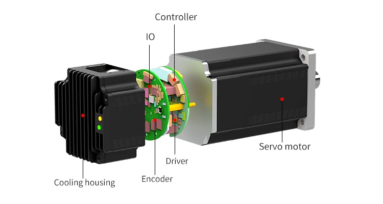
Figure: Integrated (drive-in-one) servo motor — the driver is integrated into the motor's rear end cap, and three-loop computation is completed inside the motor

Taking Limaisheng NiMotion's PMM60 series integrated servo motor as an example:

The engineering value this brings:

• Wiring drops from a dozen-plus cables to 2–3 (power + communication);

• No driver mounting space or heat dissipation design needed in the cabinet;

• The encoder cable disappears entirely, greatly reducing EMC problems;

• Supports power-limiting function, automatic gain switching, and single-turn/multi-turn absolute position recovery.